通常情况下说 Prometheus 可能只是指“Prometheus 指标”或者“Prometheus 告警”，而不是单纯的 Prometheus Server。完整的 Prometheus 是一个由多种组件组成的体系，每种组件都有其特定的应用场景，它们之间的关系如下图所示。

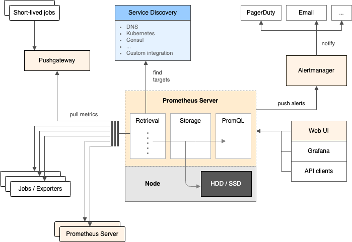
组件功能概览

Prometheus（Server）：

• 数据存储: Prometheus 是一个时序数据库（这是其最核心的功能），用于存储指标数据，同时有自己的查询语言（PromQL），用于查询和分析指标数据。
• 指标抓取: Prometheus 会定期抓取被监控实例公开的所有指标数据，抓取后将他们按照时间顺序存储起来。
• 发出告警: Prometheus 会定期执行给定的规则，规则一般通过 PromQL 查询数据，并在满足规则中定义的条件时向 Alertmanager 发出告警（每次评估规则时，只要满足告警条件就会发送告警）。

Alertmanager:

Prometheus 只管根据指标以及告警条件发出告警，之后由 Alertmanager 组件来管理这些告警。

• 警告通知: 将告警信息发送给告警接收人。
• 告警抑制: 一般情况下，Prometheus 会持续发送告警，但是 Alertmanager 并不会每次受到告警都将告警发送给告警接收人，因为此告警可能已经通知过了。
• 告警恢复: 如果 Alertmanager 持续一段时间没有再受到 Prometheus 的告警信息，则 Alertmanager 就认为对应告警已经恢复。

UI:

UI 是指 WEB UI 或 Prometheus API 客户端，通过他们可以以可视化的方式和 Prometheus 进行交互。

PushGateway:

正常情况下，Prometheus 都是采用定期主动抓取的方式，但是有些场景不能使用这种方式，比如存在周期很短的云函数等。在这种情况下就不能直接通过 Prometheus 直接去抓取，以云函数为例，可以让函数运行期间将其相关的指标信息主动推送到 PushGateway，这样，当 Prometheus 去抓取 PushGateway 的时候就能拿到云函数的相关指标。

PushProx:

当 Prometheus 和被抓取的目标位于两个隔离的网络时，如果能从目标网络访问到 Prometheus 网络，但是不能从 Prometheus 网络访问到目标网络时（典型案例是：Prometheus 位于公网，而被抓取目标位于内网），官方提供的一个解决方案。通过 PushProx，可以让 Prometheus 访问到防火墙后的目标实例，从而实现主动抓取行为。实际使用中不一定要通过这种方式，只要能让 Prometheus 能抓取到目标指标即可。

Service Discovery:

Service Discovery（服务发现）并不是 Prometheus 项目的组件，而只是让 Prometheus 自动发现被抓取目标的方式之一。Prometheus 支持多种方式的服务发现。

Prometheus 体系常用模块示例。

Prometheus

安装

cat > prometheus.yml <<EOF
# my global config
global:
  scrape_interval: 15s # 将抓取间隔设置为每 15 秒。默认为每 1 分钟。
  evaluation_interval: 15s # 每 15 秒评估一次规则。默认值为每 1 分钟。
  # scrape_timeout 设置为全局默认值 (10s)。

  # 与外部系统（联合、远程存储、Alertmanager）通信时将这些标签附加到任何时间序列或警报。
  external_labels:
    monitor: 'codelab-monitor'

# Alertmanager 配置
alerting:
  alertmanagers:
    - static_configs:
        - targets:
          # - alertmanager:9093

# 加载规则一次并根据全局“evaluation_interval”定期对其进行评估。
rule_files:
  # - "first_rules.yml"
  # - "second_rules.yml"

# 一个抓取配置只包含一个要抓取的端点
scrape_configs:
  # 里是 Prometheus 本身。
  # 作业名称作为标签`job=<job_name>`添加到从此配置中抓取的任何时间序列。
  - job_name: "prometheus"

    # metrics_path 默认为 '/metrics'
    # scheme 默认为 'http'.

    static_configs:
      - targets: ["localhost:9090"]
EOF

PWD=$(dirname $(readlink -f "$0"))

docker run -d \
  --restart=always \
  --name prometheus \
  -p 9090:9090 \
  -v /etc/localtime:/etc/localtime \
  -v ${PWD}/prometheus:/prometheus `# 数据存储目录` \
  -v ${PWD}/prometheus.yml:/etc/prometheus/prometheus.yml `# 配置文件` \
  prom/prometheus:v2.45.6

上述命令将使用默认配置（部分配置来源于官网开始使用）启动服务端，并将自己加入监控。

使用

安装后可通过http://localhost:9090/graph进入控制台。

有关表达式语言的详细信息，请参阅表达式语言文档。

发现

Prometheus 提供了多种服务发现选项来发现抓取目标，包括 Kubernetes、Consul 和基于文件的服务发现等。

示例

基于文件的服务发现

prometheus.yml：

scrape_configs:
- job_name: 'node'
  file_sd_configs:
  - files:
    - 'targets.json'

targets.json：

[
  { "targets": ["localhost:9100"], "labels": { "job": "node" } },
  { "targets": ["localhost:9101"], "labels": { "job": "node" } }
]

在 Spring Actuator 中添加 prometheus 端点提供指标服务

Spring Boot 配置

pom.xml:

<dependency>
    <groupId>org.springframework.boot</groupId>
    <artifactId>spring-boot-starter-actuator</artifactId>
</dependency>
<dependency>
    <groupId>io.micrometer</groupId>
    <artifactId>micrometer-registry-prometheus</artifactId>
</dependency>

application.yml：

server:
  port: 8080
  servlet:
    context-path: /project-name
management:
  endpoints:
    web:
      exposure:
        include:
          - prometheus # 公开 Prometheus 指标
  metrics:
    tags:
      application: ${spring.application.name}

现在可以通过/project-name/actuator/prometheus访问公开的指标。

统计 Controller：

@RestController
@io.micrometer.core.annotation.Timed(value = "http_api_request_duration", description = "接口响应时间", histogram = true)
public class Controller {}

手动统计Counter 指标：

public class MyClass {

    private final Counter counter;

    public MyClass(MeterRegistry registry) {
        // 创建指标实例
        this.counter = Counter
                .builder("http_api_request_count")
                .description("HTTP 接口总请求次数")
                .tags("tag-1", "value-1", "tag-2", "value-2")
                .register(registry);
    }

    public void run() {
        // 增加指标计数
        this.counter.increment();
    }
}

Prometheus 配置

由于指标路径不是常见的 /metrics 格式，而是 /project-name/actuator/prometheus 格式（前缀根据项目的不同而不同），所以指标路径需要动态生成。

假设自动发现文件为 sd-node.json:

[
  {
    "targets": ["10.10.1.3:8081"],
    "labels": { "project":"my-project" }
  }
]

即根据project标签来标识项目名，则 prometheus.yml 中关于自动发现部分的配置为：

scrape_configs:
  - job_name: spring-actuators
    # 由于抓取路径随项目变化而变化，所以动态生成（使用自动发现文件配置的属性来生成）
    relabel_configs:
      # 此配置的含义: 使用正则匹配输入数据（'source_labels: [project]'），匹配后按'replacement'的规则进行替换，并将替换后的内容写入'__metrics_path__'标签
      # 1. `__metrics_path__`为实际指标抓取是使用的路径（不含主机部分）；2. `project` 为自动发现文件`conf.d/sd-ibox-spring-dev.json` 中配置的自定义标签；3. 所有可用的标签可以通过`/service-discovery`页面查看
      - source_labels: [project]
        regex: '(.*)'
        target_label: __metrics_path__
        replacement: '/$1/actuator/prometheus'
    # 使用文件来发现抓取目标 - https://prometheus.io/docs/guides/file-sd/
    file_sd_configs:
      - files: ['sd-node.json']
        refresh_interval: 30s

如果没有 context-path，则直接通过 metrics_path: /actuator/prometheus 配置即可。

指标类型

counter（计数器）

在 Prometheus 中，计数器是一种单调递增的指标（即该值不能比前一个值减少，但可以重置），通常用于统计某个事件发生的次数。例如：

• HTTP 请求的总次数
• 错误的发生次数
• 系统启动以来的运行时间

计数器通常配合rate函数使用。

gauge（仪表）

仪表是一个可以上升或下降的数字。它可以用于衡量指标，如集群中的 Pod 数量、队列中的事件数量等。

PromQL 函数，如 max_over_time、 min_over_time 和 avg_over_time 可用于仪表指标。

histogram（直方图）

直方图可用于任何可计算的值，这些值根据桶值进行计数。存储桶边界可由开发人员配置。一个常见的示例是回复请求所需的时间，称为延迟。

示例：假设我们想要观察处理 API 请求所花费的时间。直方图不是存储每个请求的请求时间，而是允许我们将它们存储在存储桶中。例如，我们为所花费的时间定义存储桶 lower or equal 0.3、 le 0.5、 le 0.7、 le 1和 le 1.2。因此，这些是我们的存储桶，一旦计算出请求所花费的时间，它就会被添加到存储桶边界高于测量值的所有存储桶的计数中。

假设第一次请求“/ping”端点时耗时 0.25 秒，则存储桶的计数值将为：

注意：默认情况下会添加 +Inf 存储桶。

假设第二次请求“/ping”端点时耗时 0.4 秒，则存储桶的计数值将为。

由于 0.4 低于 0.5，因此达到该边界的所有桶都会增加其计数。

计数器通常配合histogram_quantile函数使用。

summary（总和）

总和还可以测量事件，并且是直方图的替代方法。它们更轻量级，但会丢失更多数据。它们是在应用程序级别计算的，因此无法聚合来自同一进程的多个实例的指标。当事先不知道指标的存储桶时，会使用直方图，但强烈建议尽可能使用直方图而不是总和。

PromQL

PromQL (Prometheus Query Language) 是 Prometheus 自己开发的数据查询 DSL 语言，语言表现力非常丰富，内置函数很多，在日常数据可视化以及rule 告警中都会使用到它。

在页面 http://localhost:9090/graph 中，输入下面的查询语句，查看结果，例如：

http_requests_total{code="200"}

字符串和数字

字符串: 在查询语句中，字符串往往作为查询条件 labels 的值，和 Golang 字符串语法一致，可以使用 "", '', 或者 ``` `, 格式如：

"this is a string"
'these are unescaped: \n \\ \t'
`these are not unescaped: \n ' " \t`

正数，浮点数: 表达式中可以使用正数或浮点数，例如：

3
-2.4

查询结果类型

PromQL 查询结果主要有 3 种类型：

• 瞬时数据 (Instant vector): 包含一组时序，每个时序只有一个点，例如：http_requests_total
• 区间数据 (Range vector): 包含一组时序，每个时序有多个点，例如：http_requests_total[5m]
• 纯量数据 (Scalar): 纯量只有一个数字，没有时序，例如：count(http_requests_total)

查询条件

Prometheus 存储的是时序数据，而它的时序是由名字和一组标签构成的，其实名字也可以写出标签的形式，例如 http_requests_total 等价于 {name="http_requests_total"}。

一个简单的查询相当于是对各种标签的筛选，例如：

http_requests_total{code="200"} // 表示查询名字为 http_requests_total，code 为 "200" 的数据

查询条件支持正则匹配，例如：

http_requests_total{code!="200"}  // 表示查询 code 不为 "200" 的数据
http_requests_total{code=～"2.."} // 表示查询 code 为 "2xx" 的数据
http_requests_total{code!～"2.."} // 表示查询 code 不为 "2xx" 的数据

操作符

Prometheus 查询语句中，支持常见的各种表达式操作符，例如

算术运算符:

支持的算术运算符有 +，-，*，/，%，^, 例如 http_requests_total * 2 表示将 http_requests_total 所有数据 double 一倍。

比较运算符:

支持的比较运算符有 ==，!=，>，<，>=，<=, 例如 http_requests_total > 100 表示 http_requests_total 结果中大于 100 的数据。

逻辑运算符:

支持的逻辑运算符有 and，or，unless, 例如 http_requests_total == 5 or http_requests_total == 2 表示 http_requests_total 结果中等于 5 或者 2 的数据。

聚合运算符:

支持的聚合运算符有 sum，min，max，avg，stddev，stdvar，count，count_values，bottomk，topk，quantile，, 例如 max(http_requests_total) 表示 http_requests_total 结果中最大的数据。

注意，和四则运算类型，Prometheus 的运算符也有优先级，它们遵从（^）> (*, /, %) > (+, -) > (==, !=, <=, <, >=, >) > (and, unless) > (or) 的原则。

内置函数

Prometheus 内置不少函数，方便查询以及数据格式化，例如将结果由浮点数转为整数的 floor 和 ceil，

floor(avg(http_requests_total{code="200"}))
ceil(avg(http_requests_total{code="200"}))

查看 http_requests_total 5分钟内，平均每秒数据

rate(http_requests_total[5m])

更多请参见详情。

rate

rate 函数主要用于 计算一个计数器在一段时间内的平均增长率。它在监控系统中被广泛用于计算每秒请求数、每秒错误数等指标。

rate 函数通过比较一段时间内计数器的值的变化来计算增长率。它可以帮助我们回答以下问题：

• 系统当前的负载如何？ 通过计算每秒请求数，我们可以了解系统当前承受的压力。
• 系统性能是否稳定？ 通过观察每秒错误数的趋势，我们可以判断系统是否出现了问题。
• 系统资源是否充足？ 通过计算资源使用量的增长率，我们可以预测系统是否会很快耗尽资源。

函数语法

rate(v[d])

• v: 一个计数器指标。
• d: 时间间隔，例如 5m、1h 等。

示例

rate(go_gc_duration_seconds_count[5m])

注意事项

• 计数器重置: rate 函数假设计数器不会被重置。如果计数器被重置，计算结果将不准确。
• 时间间隔: 选择合适的时间间隔非常重要。太短的时间间隔可能导致结果波动较大，太长的时间间隔可能掩盖短期内的变化。
• 采样率: rate 函数的计算结果与 Prometheus 的采样率有关。采样率越高，计算结果越精确。

常见应用场景

• 计算每秒请求数 (QPS): 监控系统负载。
• 计算错误率: 评估系统稳定性。
• 计算资源使用率: 预测系统容量。
• 检测异常: 发现系统中的异常行为。

histogram_quantile

histogram_quantile 主要用于 计算直方图指标的分位数。它在监控系统中被广泛用于计算延迟、请求大小等指标的分位数，从而更深入地了解系统的性能分布。

函数语法

histogram_quantile(φ, histogram)

• φ: 要计算的分位数，是一个介于 0 和 1 之间的浮点数。例如，0.95 表示计算第 95 个百分位数。
• histogram: 一个直方图指标。

示例

假设我们有一个名为 http_request_duration_seconds 的直方图指标，用于统计 HTTP 请求的耗时。我们可以使用以下查询来计算最近 5 分钟内请求耗时的第 99 个百分位数：

histogram_quantile(0.99, rate(http_request_duration_seconds[5m]))

函数的工作原理

histogram_quantile 函数通过以下步骤计算分位数：

1. 找到包含目标分位数的桶: 函数会找到一个桶，使得该桶以及所有小于该桶的桶中的数据点之和大于或等于目标分位数所对应的数据点数量。
2. 线性插值: 如果目标分位数落在两个桶之间，函数会使用线性插值的方法来计算精确的分位数值。

使用场景

• 计算服务延迟: 计算请求处理时间的 P95、P99 等分位数，以了解服务的性能瓶颈。
• 分析请求大小分布: 计算请求大小的分位数，以优化资源分配。
• 监控错误率: 计算错误请求比例，以了解系统的稳定性。

注意事项

• 直方图数据: 确保你的指标是直方图类型，并且具有正确的桶边界。
• 分位数范围: 分位数的值必须在 0 和 1 之间。
• 线性插值假设: histogram_quantile 函数假设桶内的数据分布是线性的，这可能导致计算结果与实际值存在一定的误差。
• rate 函数: 在计算分位数之前，通常会使用 rate 函数来计算一段时间内的平均增长率，以获得更准确的结果。

常见问题

• 为什么我计算的 P99 值总是比预期的要高？
  • 这可能是因为你的桶边界设置不合理，导致数据点集中在几个桶中。
  • 也可以是因为你的样本数量不够多，导致统计结果不够准确。
• 如何选择合适的桶边界？
  • 桶边界的选择取决于你想要分析的数据的分布情况。一般来说，对于长尾分布的数据，需要设置更多的桶边界。

常用 PromQL

磁盘相关

• 查询剩余空间

  node_filesystem_free_bytes{job="node-hx", fstype=~"xfs|ext4", mountpoint!~"/boot.*"}
  

• 查询总空间

  node_filesystem_size_bytes{job="node-hx", fstype=~"xfs|ext4", mountpoint!~"/boot.*"}
  

• 查询已用空间百分比

  // (1 - 剩余空间 / 总空间) * 100
  (1 - node_filesystem_free_bytes{job="node-hx", fstype=~"xfs|ext4", mountpoint!~"/boot.*"} / node_filesystem_size_bytes{job="node-hx", fstype=~"xfs|ext4", mountpoint!~"/boot.*"}) * 100
  

PushProx

PushProx 是一个客户端和代理，用于解决 Prometheus 无法直接对抓取位于 NAT 后面的监控实例问题（即只能能从一端访问另一端，如果双方都不不能相互访问时不使用使用此种方式）。

使用

服务端

服务端运行环境需要能被 Prometheus 访问，同时也需要能被 客户端访问（通常和 Prometheus 在一起）。

./pushprox-proxy

服务端默认监听 8080 端口.

客户端

./pushprox-client --proxy-url=http://proxy:8080/ --fqdn=<clientName>

常用参数:

--proxy-url: 服务端地址。

--fqdn: 客户端名称。可选，如果缺省则会使用客户端主机名，该名称用于 Prometheus 抓取时指定的客户端 Host。

Prometheus 使用

scrape_configs:
- job_name: node
  proxy_url: http://proxy:8080/
  static_configs:
    - targets: ['<clientName>:9100']

抓取时使用proxy_url指定代理服务器地址，同时抓取的目标中使用代理客户端fqdn的名称作为目标Host。

Alertmanager

使用 Prometheus 发出警报分为两部分。中的警报规则 Prometheus 服务器向 Alertmanager 发送警报。警报 管理器 然后管理这些警报，包括静音、抑制、聚合和 通过电子邮件、待命通知系统和聊天平台等方式发送通知。

设置警报和通知的主要步骤是：

• 设置和 配置 Alertmanager

• 配置 Prometheus 以与 Alertmanager 通信

• 告警规则 在 Prometheus 中创建

See. https://prometheus.io/docs/alerting/latest/overview/

See. https://prometheus.io/docs/alerting/latest/configuration

接收器

即告警通知接收人，可以是 webhook、邮件、短信等。

WebHook

示例：

global:
  resolve_timeout: 5m
route:
  receiver: webhook_receiver
receivers: # 可以定义多个接收者
    - name: webhook_receiver # 接收者名称，名称可以随意
      webhook_configs:
        - url: 'https://webhook.site/2c6de686-efd7-4f8e-9e8f-7838f36a9b25' # 当告警产生后，将相关信息发送到该 URL
          send_resolved: false # 当恢复后是否发送恢复通知

Grafana

https://grafana.com/docs/grafana

OpenMetrics

OpenMetrics，是云原生、高度可扩展的指标协议。 OpenMetrics 定义了大规模上报云原生指标的事实标准，并支持文本表示协议和 Protocol Buffers 协议。

Micrometer指标类型

相关文档

• Spring Boot应用如何快速接入Prometheus监控
• Loki - 日志组件